Ansys HFSS Analysis on SyncHPC

Ansys HFSS delivers 3-D full-wave accuracy for components to enable RF and high-speed design. Many times, HFSS needs High Performance Computing (HPC) infrastructure for complex problems. This blog post presents the performance of projects executed on Ansys HFSS using SyncHPC. In this experiment, team tried to design and analyze printed slotted antenna with dielectric hyperboloid lens.

Analysis by Direct Solver:

Selected project is configured to be solved by “Direct solver”.  A single machine with 128GB RAM could not start the HFSS solver on Single CPU core. The same project is successfully converged on SyncHPC based HPC cluster with each node with 224GB RAM.

The results of time taken for each configuration for first 2 adaptive passes is listed below:

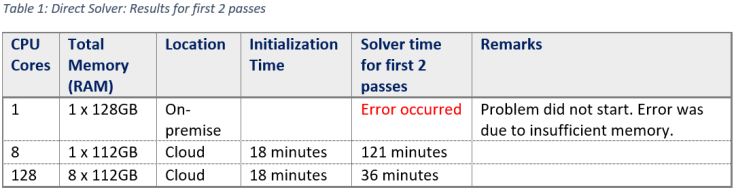Even with 8 x 112GB memory, an error occurred at 5^th Adaptive pass. The error was due to insufficient memory. Team changed the configuration to 224GB per node of HPC.

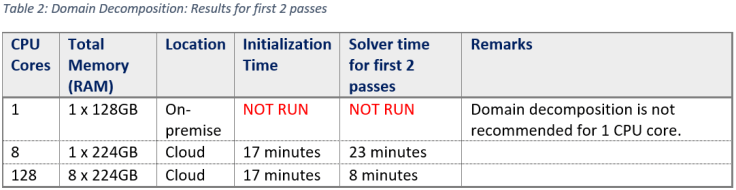
Analysis by Domain Decomposition

Later the project is configured to be solved by “Domain Decomposition” method. This is recommended for HPC configuration. Also, the Memory of each machine in Cloud is increased to 224GB. Following tables lists the results for first 2 adaptive passed using Domain decomposition method.

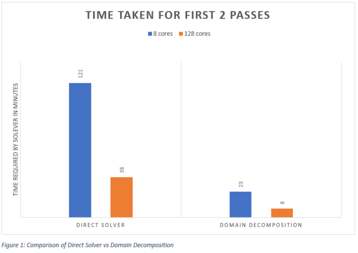
Following figure shows the comparison between Direct Solver vs Domain Decomposition.

Note: As the iteration count increases, the number of elements to be solved also increase. Hence, time required to solve those elements is more for higher iteration count. The effectiveness of HPC machines will be better for higher number of iterations.

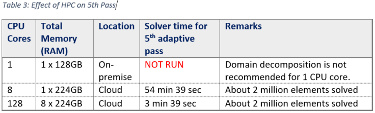
Next table shows the effect of HPC for 5^th Adaptive pass. There are couple of reasons to specifically mention results for this pass:

1. Using 8 CPU cores, there was an error in 6^th Adaptive pass. It was due to insufficient distributed memory.
2. The effect of HPC is significant as the adaptive pass count increases.

Below table shows the results of completely converged solution. As shown in table, 8 CPU core machine could not solve the problem beyond 5^th pass. It was due to insufficient memory.

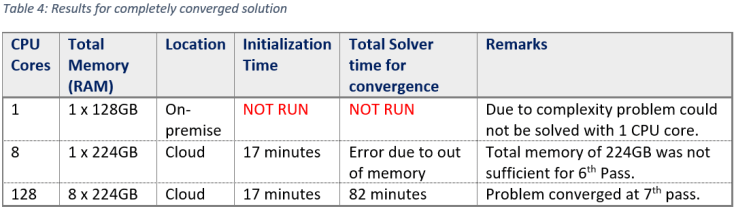
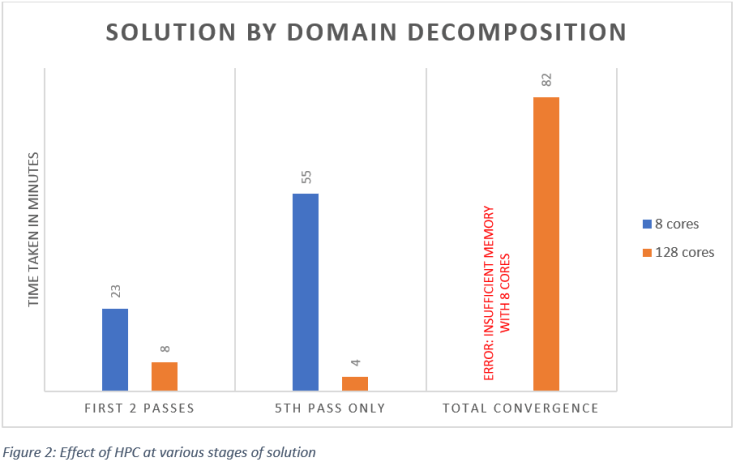
Figure 2 compares two HPC configurations (8 cores vs 128 cores) at various stages of the solution.

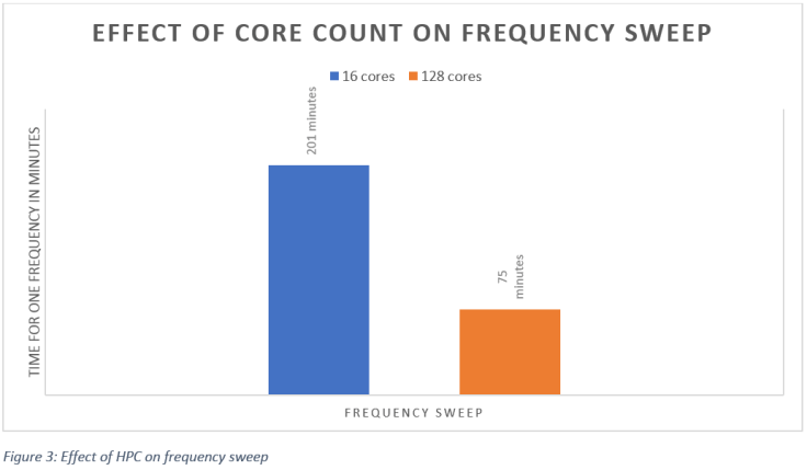
Frequency Sweep

The project was configured with the frequency sweep from frequencies 4.81GHz to 6.81GHz with 200 steps. Full solution of one of frequencies was executed on 16 cores and 128 cores respectively. The results are shown in following figure:

Concluding Remarks

Team tried to solve the problem by various configurations as mentioned in this report. Here is the summary of conclusion derived from these experiments:

• Cloud computing helped to dynamically increase size of Memory and number of CPU cores with very low turnaround time.

Memory size of 112GB per machine is not sufficient to solve this problem. The cloud machines were “re-configured” to use 224GB of memory within few minutes. It could not have been possible with physical machines in the labs.

• The number of machines are dynamically changed based on number of CPU requirements. E.g. earlier experiments were done on 8 CPU cores and then they were executed on 128 CPU cores.
• The solution of problem did not even start with 1 CPU core.
• The solution started with 8 CPU cores. But, error occurred at later passes due to insufficient memory.
• The problem could be solved successfully with 128 CPU cores.
• The performance of 128 CPU cores is far better than 8 CPU cores. The effect of higher number of CPU cores is predominant for higher number of passes. E.g. 8 CPU cores took almost 55 minutes to execute 5^th But, 128 CPU cores required less than 4 minutes to execute 5^th Pass.
• ‘Domain Decomposition solution’ is recommended over ‘Direct Solver’ for HPC configuration.