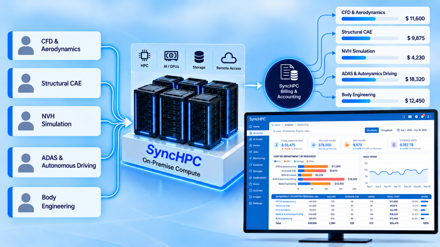
The GPU is busy. The cluster is busy. The queue is busy. But who is actually consuming the compute, and what is that consumption costing the organization?
That question gets harder when one infrastructure serves HPC simulations, AI workloads, remote engineering labs, VDI, and containerized applications. A single GPU may run a Slurm job overnight, serve an AI workload through Kubernetes during the day, and be reached through a remote lab by another team.
Modern organizations are moving from dedicated, department-owned infrastructure to shared pools of CPU, GPU, HPC, Kubernetes, VDI, storage, and visualization resources.
The shift: Machine Ownership → Compute Consumption.
As HPC, AI, and remote labs converge into a shared infrastructure, organizations need visibility into who consumed which resources, for what workload, and at what cost.
The user experience can remain simple:
Login → Select Environment → Submit Work → Use Compute → Disconnect
Behind the scenes, the platform must track users, projects, CPU/GPU hours, memory, storage, applications, MIG partitions, and access modes.
Scheduling tells you what is running. Monitoring tells you what is happening. Accounting tells you who consumed what. Showback/chargeback connects consumption to organizational cost.
Utilization tells you a resource is being used. It doesn’t tell you who used it, why, or what it cost. That gap between utilization and compute economics is what this post is about.
One Management Layer for Shared Compute
Schedulers like Slurm and Kubernetes each know their own workloads. Neither gives a unified view of the shared environment. SyncHPC is the management layer above them, connecting users and workloads to the infrastructure underneath:
Users / Researchers / Engineers / Students
↓
SyncHPC
↓
Slurm | Kubernetes | Remote Labs | VDI
↓
CPU | GPU | Storage | Applications
↓
Usage & Accounting
↓
Showback / Chargeback
The goal is one infrastructure, one consumption view, one cost model.
What SyncHPC Brings to a Compute-Oriented Campus
- Hybrid by design. The same platform manages HPC and VDI across on-premises, Azure, AWS, and GCP, so cloud bursting and on-prem clusters don’t become separate silos with separate reports.
- HPC and remote labs together. Batch jobs and interactive VDI sessions are managed in one place. That matters because a remote lab session and a Slurm job can consume the same GPU.
- Application awareness. Engineering workloads run on solvers such as Fluent, Abaqus, LS-DYNA, Nastran, and OptiStruct. Knowing which application drove the usage is what turns a job ID into a meaningful cost line.
- AI Assist before submission. SyncHPC can predict job parameters before a job is submitted. This is a natural fit for planning, since users and administrators can see what a run is likely to need before it consumes anything.
From Machine Ownership to Compute Consumption
Traditionally, a department bought servers and a lab bought workstations. Infrastructure belonged to whoever used it.
Today, CPU-based HPC, GPU-heavy AI, CAE simulation, VDI, and Kubernetes workloads share one pool across departments, researchers, students, and projects. The question shifts from “Which workstation belongs to this engineer?” to “How much compute did this user, project, or department consume?”
From Utilization to Consumption Accounting
- Scheduling tells you what is running.
- Monitoring tells you what is happening.
- Accounting tells you who consumed what.
Take a shared pool of 20 GPUs. A dashboard says they’re highly utilized. Leadership needs more: Department A used 42% of GPU capacity, Research Group B 31%, Engineering Team C 18%. And what did that consumption cost?
Building the Cost Model
Consumption covers more than CPU hours:
| Resource | Example Unit |
| CPU | CPU-hour |
| GPU / MIG partition | GPU-hour / partition-hour |
| Memory | GB-hour |
| Storage | GB-month |
| Remote desktop | Session-hour |
| Application licenses | License-hour |
The workflow has four steps:
- Identify the consumer: user, project, department, grant, or cost center.
- Capture usage: for example, User A used 120 CPU-hours, 14 GPU-hours, and 250 GB of storage.
- Apply internal rates: CPU × ₹X, GPU × ₹Y, storage × ₹Z.
- Report and allocate by user, project, department, application, cluster, or time period.
The result is a traceable chain: User → Project → Department → Resources → Usage → Cost. For engineering teams it can extend to Engineer → Project → Application → Compute → License → Cost.
Showback vs. Chargeback
Showback gives visibility without billing: “Engineering consumed ₹8.4 lakh of compute this quarter.” It supports transparency and responsible usage.
Chargeback allocates that consumption to a department, project, customer, grant, or cost center. In a university, that could mean research grants, labs, courses, or external projects.
The infrastructure doesn’t change. What changes is the link between consumption and accountability. Many organizations start with showback and move to chargeback later.
Better Capacity Planning
Consumption data does more than allocate cost. Instead of saying “We need more GPUs,” you can say: “GPU demand grew X%, driven by Projects A and B consuming Y GPU-hours. Adding Z GPUs would cover the projected demand.” That is a measurable case for investment.
Conclusion
Compute-oriented campuses will be defined not just by how much compute they deliver, but by how well it is shared, managed, measured, and accounted for. Showback and chargeback provide the economic layer, and SyncHPC provides the management and visibility layer that connects users and workloads to shared HPC and hybrid infrastructure.
SyncHPC: Manage. Monitor. Account. Optimize.


Leave a Reply